\ie \cf

$\newcommand{\norm}[1]{\\|#1\\|} \newcommand{\tr}{\text{tr}} \newcommand{\mor}{\text{Mor}} \newcommand{\hom}{\text{Hom}} \newcommand{\id}{\text{id}} \newcommand{\obj}{\text{obj}} \newcommand{\pr}{\text{pr}} \newcommand{\ker}{\text{ker}} \newcommand{\coker}{\text{coker}} \newcommand{\im}{\text{im}} \newcommand{\bbA}{\mathbb A} \newcommand{\bbB}{\mathbb B} \newcommand{\bbC}{\mathbb C} \newcommand{\bbD}{\mathbb D} \newcommand{\bbE}{\mathbb E} \newcommand{\bbF}{\mathbb F} \newcommand{\bbG}{\mathbb G} \newcommand{\bbH}{\mathbb H} \newcommand{\bbI}{\mathbb I} \newcommand{\bbJ}{\mathbb J} \newcommand{\bbK}{\mathbb K} \newcommand{\bbL}{\mathbb L} \newcommand{\bbM}{\mathbb M} \newcommand{\bbN}{\mathbb N} \newcommand{\bbO}{\mathbb O} \newcommand{\bbP}{\mathbb P} \newcommand{\bbQ}{\mathbb Q} \newcommand{\bbR}{\mathbb R} \newcommand{\bbS}{\mathbb S} \newcommand{\bbT}{\mathbb T} \newcommand{\bbU}{\mathbb U} \newcommand{\bbV}{\mathbb V} \newcommand{\bbW}{\mathbb W} \newcommand{\bbX}{\mathbb X} \newcommand{\bbY}{\mathbb Y} \newcommand{\bbZ}{\mathbb Z} \newcommand{\cA}{\mathcal A} \newcommand{\cB}{\mathcal B} \newcommand{\cC}{\mathcal C} \newcommand{\cD}{\mathcal D} \newcommand{\cE}{\mathcal E} \newcommand{\cF}{\mathcal F} \newcommand{\cG}{\mathcal G} \newcommand{\cH}{\mathcal H} \newcommand{\cI}{\mathcal I} \newcommand{\cJ}{\mathcal J} \newcommand{\cK}{\mathcal K} \newcommand{\cL}{\mathcal L} \newcommand{\cM}{\mathcal M} \newcommand{\cN}{\mathcal N} \newcommand{\cO}{\mathcal O} \newcommand{\cP}{\mathcal P} \newcommand{\cQ}{\mathcal Q} \newcommand{\cR}{\mathcal R} \newcommand{\cS}{\mathcal S} \newcommand{\cT}{\mathcal T} \newcommand{\cU}{\mathcal U} \newcommand{\cV}{\mathcal V} \newcommand{\cW}{\mathcal W} \newcommand{\cX}{\mathcal X} \newcommand{\cY}{\mathcal Y} \newcommand{\cZ}{\mathcal Z} \newcommand{\rmA}{\mathfrak A} \newcommand{\rmB}{\mathfrak B} \newcommand{\rmC}{\mathfrak C} \newcommand{\rmD}{\mathfrak D} \newcommand{\rmE}{\mathfrak E} \newcommand{\rmF}{\mathfrak F} \newcommand{\rmG}{\mathfrak G} \newcommand{\rmH}{\mathfrak H} \newcommand{\rmI}{\mathfrak I} \newcommand{\rmJ}{\mathfrak J} \newcommand{\rmK}{\mathfrak K} \newcommand{\rmL}{\mathfrak L} \newcommand{\rmM}{\mathfrak M} \newcommand{\rmN}{\mathfrak N} \newcommand{\rmO}{\mathfrak O} \newcommand{\rmP}{\mathfrak P} \newcommand{\rmQ}{\mathfrak Q} \newcommand{\rmR}{\mathfrak R} \newcommand{\rmS}{\mathfrak S} \newcommand{\rmT}{\mathfrak T} \newcommand{\rmU}{\mathfrak U} \newcommand{\rmV}{\mathfrak V} \newcommand{\rmW}{\mathfrak W} \newcommand{\rmX}{\mathfrak X} \newcommand{\rmY}{\mathfrak Y} \newcommand{\rmZ}{\mathfrak Z} \newcommand{\paren}[1]{( #1 )} \newcommand{\Paren}[1]{\left( #1 \right)} \newcommand{\bigparen}[1]{\bigl( #1 \bigr)} \newcommand{\Bigparen}[1]{\Bigl( #1 \Bigr)} \newcommand{\biggparen}[1]{\biggl( #1 \biggr)} \newcommand{\Biggparen}[1]{\Biggl( #1 \Biggr)} \newcommand{\abs}[1]{\lvert #1 \rvert} \newcommand{\Abs}[1]{\left\lvert #1 \right\rvert} \newcommand{\bigabs}[1]{\bigl\lvert #1 \bigr\rvert} \newcommand{\Bigabs}[1]{\Bigl\lvert #1 \Bigr\rvert} \newcommand{\biggabs}[1]{\biggl\lvert #1 \biggr\rvert} \newcommand{\Biggabs}[1]{\Biggl\lvert #1 \Biggr\rvert} \newcommand{\card}[1]{\left| #1 \right|} \newcommand{\Card}[1]{\left\lvert #1 \right\rvert} \newcommand{\bigcard}[1]{\bigl\lvert #1 \bigr\rvert} \newcommand{\Bigcard}[1]{\Bigl\lvert #1 \Bigr\rvert} \newcommand{\biggcard}[1]{\biggl\lvert #1 \biggr\rvert} \newcommand{\Biggcard}[1]{\Biggl\lvert #1 \Biggr\rvert} \newcommand{\norm}[1]{\lVert #1 \rVert} \newcommand{\Norm}[1]{\left\lVert #1 \right\rVert} \newcommand{\bignorm}[1]{\bigl\lVert #1 \bigr\rVert} \newcommand{\Bignorm}[1]{\Bigl\lVert #1 \Bigr\rVert} \newcommand{\biggnorm}[1]{\biggl\lVert #1 \biggr\rVert} \newcommand{\Biggnorm}[1]{\Biggl\lVert #1 \Biggr\rVert} \newcommand{\iprod}[1]{\langle #1 \rangle} \newcommand{\Iprod}[1]{\left\langle #1 \right\rangle} \newcommand{\bigiprod}[1]{\bigl\langle #1 \bigr\rangle} \newcommand{\Bigiprod}[1]{\Bigl\langle #1 \Bigr\rangle} \newcommand{\biggiprod}[1]{\biggl\langle #1 \biggr\rangle} \newcommand{\Biggiprod}[1]{\Biggl\langle #1 \Biggr\rangle} \newcommand{\set}[1]{\lbrace #1 \rbrace} \newcommand{\Set}[1]{\left\lbrace #1 \right\rbrace} \newcommand{\bigset}[1]{\bigl\lbrace #1 \bigr\rbrace} \newcommand{\Bigset}[1]{\Bigl\lbrace #1 \Bigr\rbrace} \newcommand{\biggset}[1]{\biggl\lbrace #1 \biggr\rbrace} \newcommand{\Biggset}[1]{\Biggl\lbrace #1 \Biggr\rbrace} \newcommand{\bracket}[1]{\lbrack #1 \rbrack} \newcommand{\Bracket}[1]{\left\lbrack #1 \right\rbrack} \newcommand{\bigbracket}[1]{\bigl\lbrack #1 \bigr\rbrack} \newcommand{\Bigbracket}[1]{\Bigl\lbrack #1 \Bigr\rbrack} \newcommand{\biggbracket}[1]{\biggl\lbrack #1 \biggr\rbrack} \newcommand{\Biggbracket}[1]{\Biggl\lbrack #1 \Biggr\rbrack} \newcommand{\ucorner}[1]{\ulcorner #1 \urcorner} \newcommand{\Ucorner}[1]{\left\ulcorner #1 \right\urcorner} \newcommand{\bigucorner}[1]{\bigl\ulcorner #1 \bigr\urcorner} \newcommand{\Bigucorner}[1]{\Bigl\ulcorner #1 \Bigr\urcorner} \newcommand{\biggucorner}[1]{\biggl\ulcorner #1 \biggr\urcorner} \newcommand{\Biggucorner}[1]{\Biggl\ulcorner #1 \Biggr\urcorner} \newcommand{\ceil}[1]{\lceil #1 \rceil} \newcommand{\Ceil}[1]{\left\lceil #1 \right\rceil} \newcommand{\bigceil}[1]{\bigl\lceil #1 \bigr\rceil} \newcommand{\Bigceil}[1]{\Bigl\lceil #1 \Bigr\rceil} \newcommand{\biggceil}[1]{\biggl\lceil #1 \biggr\rceil} \newcommand{\Biggceil}[1]{\Biggl\lceil #1 \Biggr\rceil} \newcommand{\floor}[1]{\lfloor #1 \rfloor} \newcommand{\Floor}[1]{\left\lfloor #1 \right\rfloor} \newcommand{\bigfloor}[1]{\bigl\lfloor #1 \bigr\rfloor} \newcommand{\Bigfloor}[1]{\Bigl\lfloor #1 \Bigr\rfloor} \newcommand{\biggfloor}[1]{\biggl\lfloor #1 \biggr\rfloor} \newcommand{\Biggfloor}[1]{\Biggl\lfloor #1 \Biggr\rfloor} \newcommand{\lcorner}[1]{\llcorner #1 \lrcorner} \newcommand{\Lcorner}[1]{\left\llcorner #1 \right\lrcorner} \newcommand{\biglcorner}[1]{\bigl\llcorner #1 \bigr\lrcorner} \newcommand{\Biglcorner}[1]{\Bigl\llcorner #1 \Bigr\lrcorner} \newcommand{\bigglcorner}[1]{\biggl\llcorner #1 \biggr\lrcorner} \newcommand{\Bigglcorner}[1]{\Biggl\llcorner #1 \Biggr\lrcorner} \newcommand{\Rnn}{\bbR_{\ge 0}} \DeclareMathOperator{\Tr}{Tr} \DeclareMathOperator{\min}{min} \DeclareMathOperator{\max}{max} \DeclareMathOperator{\argmax}{arg\,max} \DeclareMathOperator{\argmin}{arg\,min} \DeclareMathOperator{\E}{\mathbb E} \DeclareMathOperator{\pE}{\tilde{\mathbb E}} \DeclareMathOperator{\Pr}{\mathbb P} \DeclareMathOperator{\Span}{Span} \DeclareMathOperator{\Cone}{Cone} \DeclareMathOperator{\Det}{\textbf{Det}} \DeclareMathOperator{\Perm}{\textbf{Perm}} \DeclareMathOperator{\Sym}{\textbf{Sym}} \DeclareMathOperator{\Pow}{\textbf{Pow}} \DeclareMathOperator{\Gal}{\textbf{Gal}} \DeclareMathOperator{\Aut}{\textbf{Aut}} \notag$

$\newcommand{\1}{\ensuremath{\mathrm{1}}} \notag$

$\newcommand{\transpose}[1]{\ensuremath{#1{}^{\mkern-2mu\intercal}}} \newcommand{\dyad}[1]{\ensuremath{#1#1{}^{\mkern-2mu\intercal}}} \newcommand{\nchoose}[1]{\ensuremath} \newcommand{\generated}[1]{\ensuremath{\langle #1 \rangle}} \notag$

\newcommand{\eqdef}{\mathbin{\stackrel{\rm def}{=}}}  \newcommand{\R} % real numbers  \newcommand{\N}} % natural numbers  \newcommand{\Z} % integers  \newcommand{\F} % a field  \newcommand{\Q} % the rationals  \newcommand{\C}{\mathbb{C}} % the complexes  \newcommand{\poly}}  \newcommand{\polylog}}  \newcommand{\loglog}}}  \newcommand{\zo}{\{0,1\}}  \newcommand{\suchthat}  \newcommand{\pr}[1]{\Pr\left[#1\right]}  \newcommand{\deffont}{\em}  \newcommand{\getsr}{\mathbin{\stackrel{\mbox{\tiny R}}{\gets}}}  \newcommand{\Exp}{\mathop{\mathrm E}\displaylimits} % expectation  \newcommand{\Var}{\mathop{\mathrm Var}\displaylimits} % variance  \newcommand{\xor}{\oplus}  \newcommand{\GF}{\mathrm{GF}}  \newcommand{\eps}{\varepsilon}  \notag

$\newcommand{\eps}{\varepsilon} \notag$

$\newcommand{\MIP}{\class{MIP}}$

\no

$\newcommand{\textprob}[1]{\text{#1}} \newcommand{\mathprob}[1]{\textbf{#1}} \newcommand{\Satisfiability}{\textprob{Satisfiability}} \newcommand{\Mor}{\textprob{Mor}} \newcommand{\Hom}{\textprob{Hom}} \newcommand{\cok}{\textprob{cok }} \newcommand{\ker}{\textprob{ker }} \newcommand{\im}{\textprob{im }} \newcommand{\coim}{\textprob{coim }} \newcommand{\id}{\textprob{id}}$

Next |

| Previous

Solving Basic Problems

100%

The Dynamic Programming Algorithm
- Principle of Optimality
- "Proof" of Validity

Now that we have set up the general framework of problems of interest, let's think about how to solve them. We begin with a standard example:

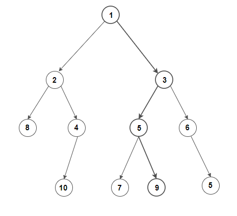
Given a directed tree with non-negative weighted nodes, find the path from root to leaf which maximizes the path sum of weights.

We could brute force this problem by looking at every path, but there is a far better approach. Consider the following pseudo-code

Input: A directed non-negative weighted tree T
for node in reverse_topological_sort T
    if node.isLeaf:
        node.path = [node]
    else:
        max_child = max(node.children on weight)
	node.weight += max_child.weight
	node.path = max_child.path + [node]
Output: root.path

This algorithm is an example of backwards recursion. The idea is that at any particular node, we can treat it as the root node, find the optimal path from that node onwards, and treat the maximum sum as the weight of the node. Thus, we can recurse backwards until we reach the root node. Amazingly, this algorithm only involves a maximum of two calls to any particular node's weights (an update and a read), vs the brute force method might call a particular node an arbitrarily large number of times.

This is a classic algorithm which appears in most algorithm textbooks, but can be generalized into an algorithm for solving general basic problems.

The Dynamic Programming Algorithm

In the example above, we saw how solving the path problem backwards helped avoid the computational complexity of the brute force approach. Let's generalize our intuition for why that process worked.

Let $\pi^*:\set{\mu_0,\ldots,\mu_{n-1}}$ be an optimal policy for the basic problem, and let $x_i$ be a state that appears with non-zero probability at time $i$ in the Markov Chain induced by the policy. Consider the problem of minimizing the "cost-to-go" from time $i$ to time $n$$$E\Set{g_n(x_n)+\sum\limits_{k=i}^{n-1}g_k(x_k,\mu_k(x_k),w_k)}$$The truncated policy $\set{\mu_i,\ldots,\mu_{n-1}}$ is optimal for this subproblem.

Suppose not: let there exist $\set{\eta_i,\ldots,\eta_{n-1}}$ optimizing the subproblem. Let $\eta^*_i$ be the action which is identical to $\eta_i$ on $x_i$ and identical to $\mu_i$ elsewhere. Then by linearity of expectation, the policy $\set{\mu_0,\ldots,\mu_{i-1},\eta^*_i,\eta_{i+1},\ldots,\eta_{n-1}}$ is optimal on the whole basic problem.

This result is useful since it now allows us to define the solution to the basic problem generally

For each time $k\in[n+1]$, define a maximal-reward function $V_k:S_k\to\Rnn$ defined by $V_n(x)=g_n(x)$ and:$$V_k(x)=\max\limits_{a\in C_k(x)}E\Bracket{g_k(x,a,P_k(\cdot\mid x,a))+V_{k+1}(P_k(\cdot\mid x,a))}$$(To ensure the definition above is well-defined, we need to define $V_k$ over probability distributions. We do so as follows: $V_k(P)=\sum V_k(y)\cdot P(x_k=y)$). Thus, the optimal policy is defined by:$$\mu_k(x)=\operatorname{argmax}\limits_{a\in C_k(x_k)}E\Bracket{g_k(x,a,P_k(\cdot\mid x,a))+V_{k+1}(P_k(\cdot\mid x,a))}$$

Applying the Principle of Optimality as the inductive step allows one to prove this result (the base case is pretty trivial). I'll leave this result as an exercise for the reader.

Notice that $V_k$ is the direct analog of weight in the example and $\mu_k$ the direct analog of path. We often call the set of $V_k$s the Bellman surface of the basic problem

To see the computational complexity of the dynamic programming algorithm, note that we have to compute all $V_k$s, and then $n$ more expected value computations to generate the optimal policy. Assuming there are $n$ time steps, no more than $m$ valid states at any time, and no more than $c$ valid actions at any time, the maximal number of $V_k$ terms to be computed is $n\cdot m\cdot c$.

Thus, an upper bound for the computational complexity of the algorithm is compute $nmc+n$ expected values. This is linear in state space size, action space size, and time.

The beauty of this algorithm is that most additional complexities (time delays, partial information, etc) can be easily dealt with by expanding the state space. However, in practice, this can lead to enormous state spaces which aren't great to work with. We'll talk about how to deal with that in the next post.

Top