Week 13 Notes
This week, we'll again be focusing on geometry.
Coordinate Geometry
In coordinate geometry, we add a coordinate grid to our geometric objects. For two-dimensional objects like circles and squares, the coordinate grid is the familiar \(x-y\) plane.
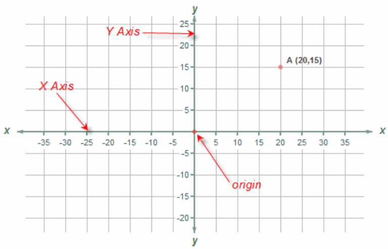
In a coordinate grid, there are two axes: the horizontal \(x\)-axis and the vertical \(y\)-axis. Both axes are real number lines, and any point in the grid is denoted by the corresponding points on the \(x\) and \(y\) axes. For example, the point \(A\) in the diagram above, if moved downwards towards the \(x\) axis, will meet the axis at value \(20\), and if moved leftwards toward the \(y\)-axis, will meet the axis at the value \(15\). So, the point is written as \((20,15)\).
The process of associating each point in the grid with \((x,y)\) coordinates is called the cartesian coordinate system. We've already seen alternate coordinate systems, like polar coordinates, in previous weeks. For now, we'll exclusively use the Cartesian system.
The origin is the point \((0,0)\). The beauty of coordinate grids is that given a geometric object, we can place the origin of the coordinate grid on the object wherever we like. We'll see examples of how that is useful soon.
Parameterizing Lines
Once we pick a coordinate system, we want to express our geometric objects as equations. Let's start by parameterizing line segments.
Given points \((a_1,b_1)\) and \((a_2,b_2)\), how do we write an equation to represent the line segment between the points?
We can think about it like a travelling problem: Suppose you are at your friend's house at point \((a_1,b_1)\), and you walk in a straight line starting at time \(t=0\) to your house at point \((a_2,b_2)\). Suppose you reach your house at time \(t=1\). At what point are you located at time \(0\leq t\leq 1\)?
The answer is the following: $$(a_2t+a_1(1-t),b_2t+b_1(1-t))$$As an example, if \((a_1,b_1)=(5,2)\) and \((a_2,b_2)=(2,5)\), the following Desmos plot will show your walking path between the two houses.
In other words, our formula for the line segment is the following: $$\{(a_2t+a_1(1-t),b_2t+b_1(1-t))\mid 0\leq t\leq 1\}$$
What about the line through the two points? The formula is quite similar:$$\{(a_2t+a_1(1-t),b_2t+b_1(1-t))\mid -\infty\lt t\lt\infty\}$$This is called the parameterization of a line.
Equations of conics
What about other shapes? How do we come up with equations for them? For polygons, we can treat the shapes as a collection of line segments. But curved surfaces are a bit more complicated.
Luckily for us, there's an important class of curved shapes that have quadratic formulas.
In other words, conics are the graphs of arbitrary quadratic polynomials. But what do they look like?
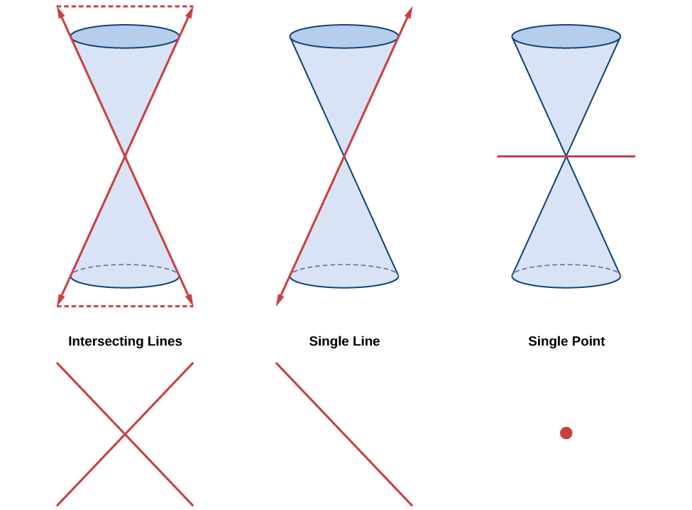
The Double Cone
The double cone is a geometric shape, composed of two infinitely tall cones that share the same vertex. It looks something like this:
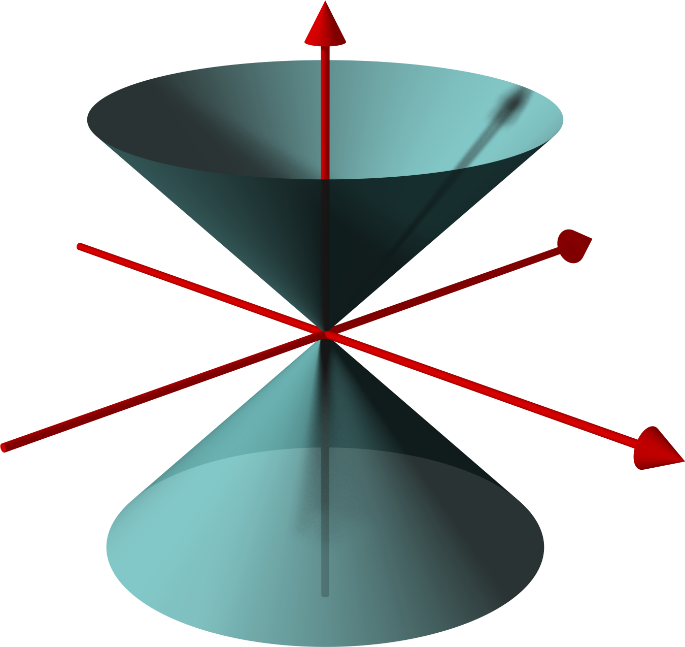
Although not pictured here, both cones go off to infinity. The double cone is quite important, since the set of shapes formed by intersecting a plane with the double cone are the conics. Here are some examples:
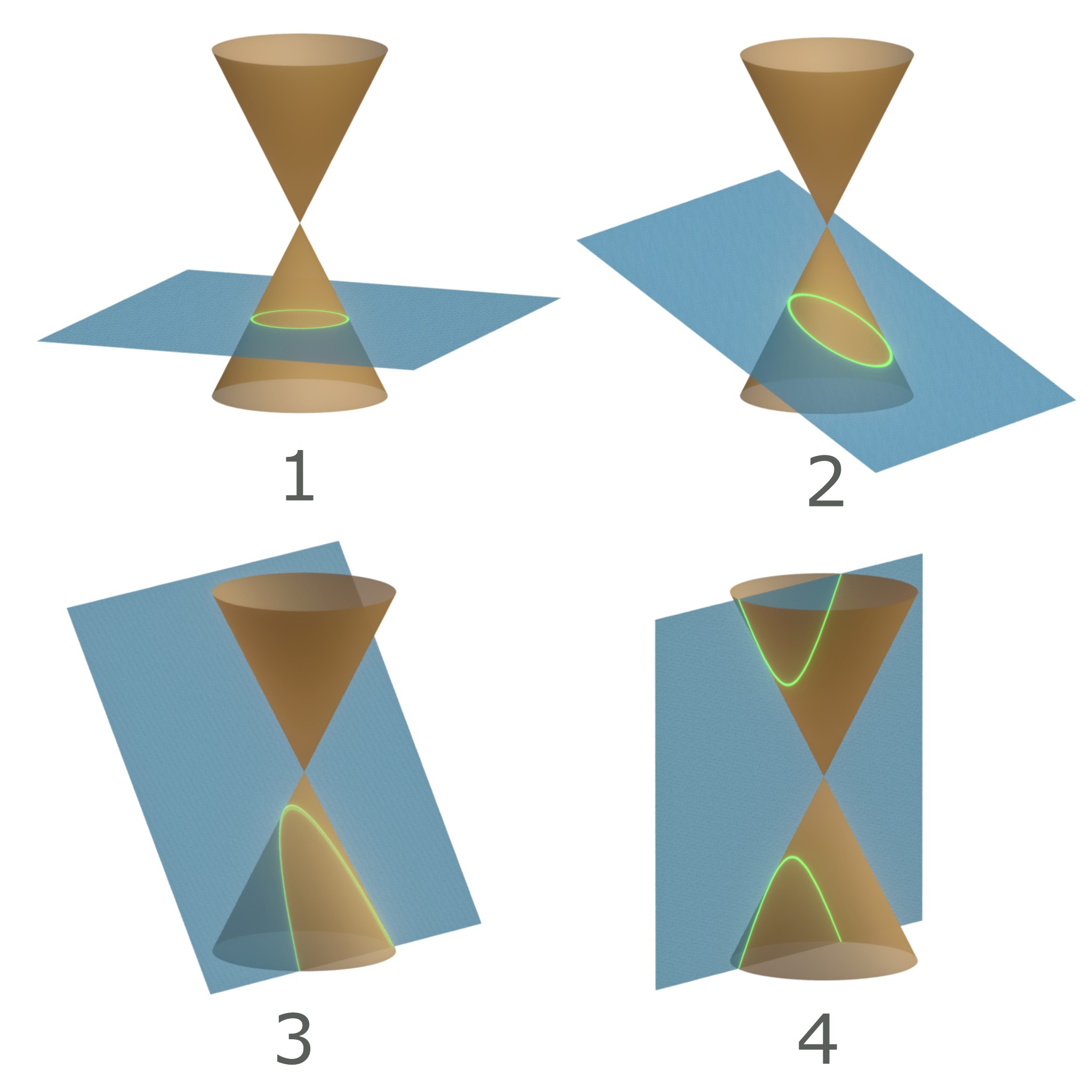
The pictured conics are
- Circle
- Ellipse
- Parabola
- Hyperbola
The circle is a type of ellipse, so really, there are only \(3\) types of conics in the picture above.
Types of Conics
Some examples of ellipses with the same diameter are as follows:
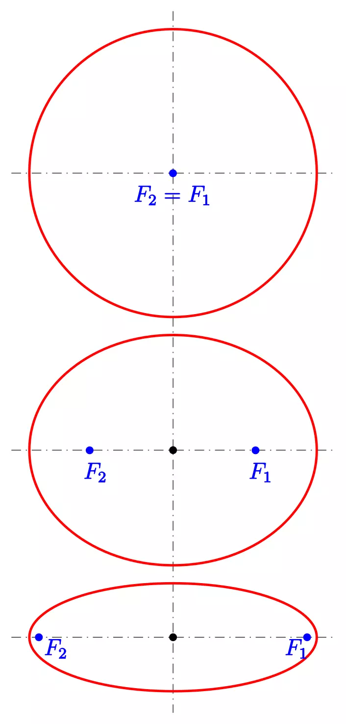
Note that when \(F_1=F_2\), we get a circle centered at the focus points. It goes without saying that the diameter must be bigger than \(\overline{F_1F_2}\) for there to be an ellipse (what happens when \(D=\overline{F_1F_2}\)?)
So what is the formula of an ellipse? If \(F_1\) and \(F_2\) are both on the \(x\)-axis (or in other words, the ellipse is horizontal), and the midpoint of \(\overline{F_1F_2}\) is the origin (or in other words, the ellipse is centered at the origin), then the formula for the ellipse is $$\frac{4x^2}{D^2}+\frac{4y^2}{D^2-\overline{F_1F_2}^2}=1$$Replacing \(\frac 4{D^2}\) with \(A\) and \(\frac4{D^2-\overline{F_1F_2}^2}\) with \(C\) gives us $$Ax^2+Cy^2=1$$where \(A,C\geq0\). This is the general form of the horizontal ellipse. The general form of the equation of an ellipse can be found here.
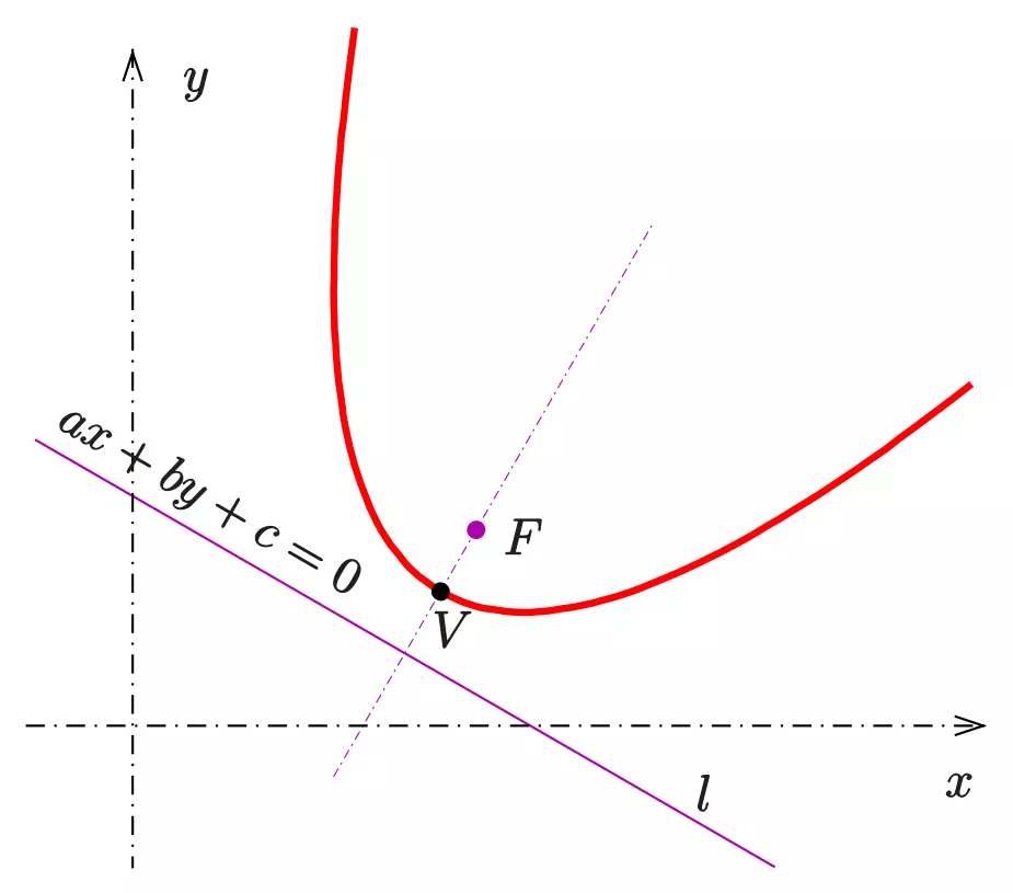
You are likely unfamiliar with this definition of a parabola, but you can easily see why it is identical to the one you are familiar with.
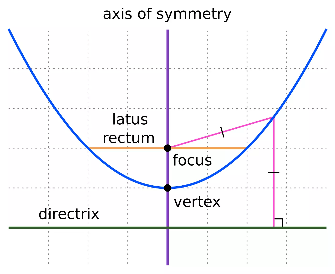
The pink lines are equal in length, showing that the distance to the focus and directrix are the same. So how do we find the formula of the parabola? We simply use the distance formula to find the distance to the focus, and then realize that the shortest distance between a line and a point is the line segment from the point perpendicular to the line. With this knowledge, we get the following formula for the parabola:
$$\frac{(ax+by+c)^2}{a^2+b^2}=(x-x_f)^2+(y-y_f)^2$$This formula is probably not that familiar, but let's set \(a=0\). Then, we get $$y^2+\frac cby+\frac{c^2}{b^2}=x^2-2xx_f+x_f^2+y^2-2yy_f+y_f^2$$$$y=\frac{b^2x^2-2b^2xx_f+b^2x_f^2+b^2y_f^2-c^2}{2b^2y_f+bc}$$Letting \(A=\frac{b^2}{2b^2y_f+bc}\), \(B=-2x_fA\), \(C=\frac{b^2x_f^2+b^2y_f^2-c^2}{2b^2y_f+bc}\), we get $$y=Ax^2+Bx+C$$Whenever the directrix is parallel to the \(x\)-axis, the formula for the parabola is the one we know well.
Hyperbolas looks like two swooshes on the same graph. The following graph plots the following hyperbolas: \(xy=1,\;xy=4,\;xy=9\).
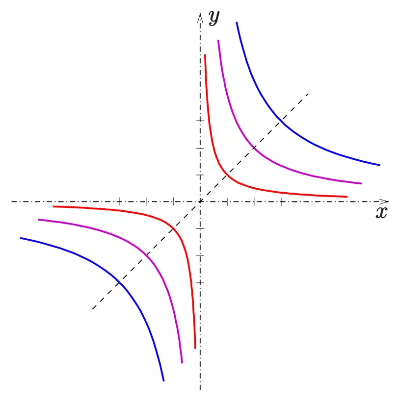
The horizontal hyperbola (the hyperbola with the \(x,y\)-axes as the lines of symmetry) has the following standard equation: $$Ax^2-Cy^2=1$$where \(A,C\geq0\).
Degenerate conics are called degenerate since their shapes don't have any curves. So given a quadratic equation \(Ax^2+Bxy+Cy^2+Dx+Ey+F=0\), how can we tell if it is an ellipse, a hyperbola, or parabola, assuming it isn't degenerate? We use the discriminant. In the quadratic equation, we use the discriminant \(b^2-4ac\) to determine whether there are \(2\) real roots, \(1\) real root, or no real roots. For conics, we have the following result:
- \(B^2-4AC>0\) implies the conic is a hyperbola
- \(B^2-4AC=0\) implies the conic is a parabola.
- \(B^2-4AC\lt0\) implies the conic is an ellipse
Dealing with Points
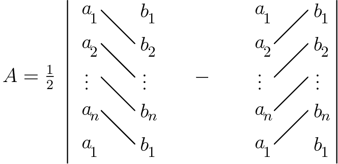
In Coordinate Geometry, we often have a collection of points, and want to either find the area of the polygon with the points as vertices, or find a polynomial that goes through the points. Luckily for us, there are ways to do both.
The shoelace theorem is named as such because the pattern of the products look like shoelaces.
- \(S_i(a_j)=0\) whenever \(i\neq j\)
- \(S_i(a_i)=b_i\)
Uniqueness: Now, we want to show that there is only one \(p\) that satisfies the desired property. Let \(f,g\) both have degree \(\lt n\) and satisfy \(f(a_i)=g(a_i)=b_i\) for all \(i\). Thus, \(a_i\) is a root of \(f-g\) for each \(i\). Thus, \((x-a_1)(x-a_2)\ldots(x-a_n)\) must be a factor of \(f-g\). Since this product has degree \(n\), which is higher than the degree of \(f-g\), \(f-g\) must be \(0\), and thus, \(f=g\).
Conclusion
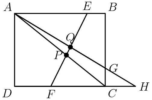
Coordinate Geometry is an alternate approach to geometry that focuses on establishing a coordinate system, and exploiting that coordinate system to find quantities that would be hard to find otherwise. The study of conics isn't all that important for competition math, but is hugely important for computation coordinate geometry, since computers use conics all the time to compute the trajectories of geometric objects. Here are an exercise that shows the difference in approach between coordinate geometry and standard geometry. Feel free to use whichever is more convenient.
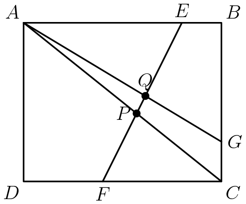
- \(AG:\;-\frac35x+4\)
- \(AC:\;-\frac45x+4\)
- \(EF:\;2x-4\)
Solution 2 (Standard Geometry): Let \(H\) be the intersection between lines \(AG\) and \(CD\)
In general, the strategy for coordinate geometry is to come up with equations for all of the important shapes (lines and curves), and then use algebra to find their points of intersection. For the remainder of these notes, we'll be focusing on the most special of conics: circles.
Circle Geometry
Let's begin our discussion of circles with some definitions.

- A secant is a line that intersects a circle at \(2\) points. A tangent is a line (segment) that intersects a circle at one point and doesn't intersect the interior of the circle.
- A chord is the line segment consisting of the points of a secant inside in the circle
- A diameter is the longest chord, and goes through the center of the circle. A radius is one half of a diameter.
We often talk about the angle subtended by a chord. By this, we mean the angle formed by the endpoints of the chord and the center of the circle, as in the following diagram:

In the diagram above, the chord \(AB\) is subtended by \(\angle AOB\). We also say that the measure of arc \(AB\), the part of the circumference of the circle between \(A\) and \(B\), is \(\angle AOB\).
If we are using radians, there is a nice formula relating the length of an arc and its measure: \(s=r\theta\). \(s\) is the length of the arc, \(r\) is the radius, and \(\theta\) is the measure of the arc in radians.
Chords of the same length have the same measure. To see why, consider the following diagram:

By SSS, both triangles are congruent, and thus the angles \(\angle AOB\) and \(\angle POQ\) are congruent.
An interior angle \(\angle APB\) is an angle with \(A,P,B\) all points on the circle. For any interior angle \(\angle APB\), the measure of the arc \(AB\) is twice \(\angle APB\), as in the following diagrams:

In each of the three cases above, \(\angle AOB=2\angle APB\). In particular, when \(\angle AOB\) is \(180^\circ\), i.e., it is a straight line, \(\angle APB\) is a right angle. So, for any right triangle, the hypotenuse will be the diameter of the circumscribing circle. The proof of this fact relies on the following diagram.
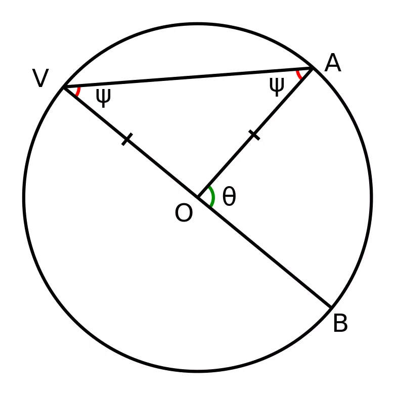
Since \(\triangle AVO\) is isosceles, \(\angle AVO=\angle VAO\), and thus \(\angle AOB=\angle AVO+\angle VAO\), so \(\angle AOB=2\angle AVO\).
Secant Theorems
There are many special relationships between secants and angles. The simplest one is that tangents are always perpendicular to the radius at the intersection point.

There are three interesting types of secant diagrams we'll look at, as shown below. \(O\) stands for the center of the circle.
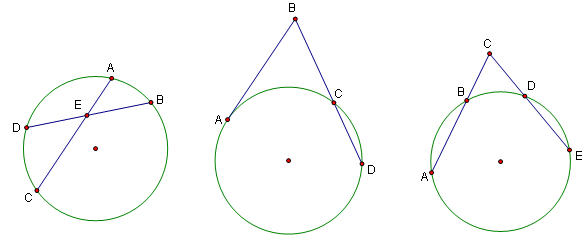
Diagram 2: Note that triangles \(\triangle ACO\), \(\triangle ADO\), and \(\triangle CDO\) are all isosceles. So, let \(\angle ACO=\angle CAO=\alpha\), \(\angle DCO=\angle CDO=\beta\), \(\angle ADO=\angle DAO=\gamma\). Since triangles have \(180^\circ\), we have $$2\alpha+2\beta+2\gamma=180^\circ\to\alpha=90^\circ-\beta-\gamma$$Since \(\angle ADC=\angle ADO+\angle CDO\), \(\angle ADC=\beta+\gamma\). So, \(\angle CAO+\angle ADC=90^\circ\). Since tangents are perpendicular to radii, \(\angle CAO+\angle BAC=90^\circ\). Thus, \(\angle BAC=\angle ADC\).
Diagram 3: Since \(\angle ACE +\angle BED=\angle ABE\), \(\angle ABE=\frac12\angle AOE\), and \(\angle BED=\frac12\angle BOD\), the desired claim is true.
Hopefully you should be able to see that these three statements are really all the same statement, just in different forms. With this theorem in hand, we can prove one of the most important theorems in circle geometry.
- There are two chords that intersect inside the circle. Thus, \(AE\cdot EC=DE\cdot EB\).
- There is a secant and tangent eminating from a point outside the circle. Thus, \(AB\cdot AB=BC\cdot BD\).
- There are two secants that intersect at a point outside the circle. Thus, \(AC\cdot BC=EC\cdot DC\).
Diagram 2: Since \(\angle ABC=\angle ABD\) and \(\angle BAC=\angle ADC\) via the Secant Angles Theorem, \(\triangle ABD\sim\triangle ABC\). So, \(\frac{AB}{AD}=\frac{BC}{AB}\). Multiplying by \(AD\cdot AB\) gives us the desired relation.
Diagram 3: Draw a tangent from point \(C\) to the circle, and apply the result from Diagram \(2\) to both secants. This completes the proof.
We often will define the power of the point as \(\overline{OP}^2-R^2\), which is identical to the definition above, except that powers of points inside the circle are negated. This gives us the following important result.
- The radical axis of \(\omega_1\) and \(\omega_2\) is a line perpendicular to \(\overline{O_1O_2}\)
- The radical axis goes through any points of intersection of the circles \(\omega_1,\omega_2\)
- There exists a unique point \(P\) on the line \(O_1O_2\) such that \(P\) is on the radical axis.
- Let \(P\) be any point in the plane, and \(P'\) the intersection of the line \(O_1O_2\) and the line perpendicular to it through \(P\). By the Pythagorean Theorem, for \(i=1,2\)$$O_iP^2=O_iP'^2+PP'^2$$Thus, \(P\) is on the radical axis if and only if \(P'\) is. When combined with the result of part \(3\), this completes the proof.
- Any point on the intersection of \(\omega_1\) and \(\omega_2\) has power \(0\) with respect to both circles, and thus is on the radical axis.
- For some point \(P\) on line \(O_1O_2\), let \(d\) be the length \(PO_1\), and \(w\) the length \(O_1O_2\). If point \(P\) is to the left of \(O_1\), then the powers of \(P\) with respect to both circles are equal if and only if $$\begin{aligned}(d+w)^2-d^2&=R_2^2-R_1^2\\d&=\frac{R_2^2-R_1^2-w^2}{2w}\end{aligned}$$If \(P\) is to the right of \(O_1O_2\), the powers of \(P\) with respect to both circles are equal if and only if $$\begin{aligned}(d-w)^2-d^2&=R_2^2-R_1^2\\-d&=\frac{R_2^2-R_1^2-w^2}{2w}\end{aligned}$$So, if \(\frac{R_2^2-R_1^2-w^2}{2w}\) is \(0\), the only point that satisfies \(d=0\) is \(O_1\). If \(\frac{R_2^2-R_1^2-w^2}{2w}\gt0\), the second equation is impossible to satisfy as \(d\geq0\), and there is exactly one point on line to the left of \(O_1\) with distance \(d\) from \(O_1\). If \(\frac{R_2^2-R_1^2-w^2}{2w}\lt0\), the first equation is impossible to satisfy as \(d\geq0\), and there is exactly one point on the line to the right of \(O_1\) with distance \(d\) from \(O_1\).
Cyclic Quadrilaterals
Any quadrilateral whose vertices are on a circle is called a cyclic quadrilateral. Cyclic quadrilaterals are defined by the following theorem.
If \(\angle ABC+\angle CDA=180^\circ\), then consider the circumcircle of \(\triangle ABC\). Call the center \(O\) and radius \(r\). There are \(3\) cases
- \(D\) is inside the circle: Let \(E\) be the other intersection of \(AD\) with the circle, and let \(F\) be the other intersection of \(CD\) with the circle. Then, by the Secant Angles Theorem, $$\angle CDA=\frac{\angle COA+\angle EOF}2=\angle BFE+\angle AFC$$So, $$\angle CDA+\angle ABC=\angle BFE+\angle AFC+\angle ABC=\angle BFE+180^\circ$$This is a contradiction.
- If \(D\) is outside the circle, then define \(E,F\) identically to the first part. Thus, $$\angle CDA=\frac{\angle AOC-\angle EOF}2=\angle AFC-\angle BFE$$So, $$\angle CDA+\angle ABC=\angle AFC-\angle BFE+\angle ABC=180^\circ-\angle BFE$$a contradiction.
- \(D\) is on the circle: This is the only possibility, finishing the theorem.
Now that we have a way to check if a quadrilateral is cyclic, we can introduce two useful theorem involving cyclic quadrilaterals.
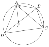
Since \(\angle ADP=\angle ADB=\angle ACB\), \(\triangle DAP\sim\triangle CAB\), so $$\frac{DP}{BC}=\frac{AD}{AC}$$Also, \(\angle APB=\angle180^\circ-\angle APD=180^\circ-\angle ABC=\angle ADC\) and \(\angle ABP=\angle ACD\), so \(\triangle APB\sim\triangle ADC\). Hence,$$\frac{BP}{CD}=\frac{AB}{AC}$$Combining these equations gives us$$\frac{BC\cdot AD+AB\cdot CD}{AC}=BP+DP=BD$$Multiplying by \(AC\) gives us Ptolemy's Theorem.
Challenge: Projective Geometry
Projective Geometry is a very important concept, but likely one you haven't seen in mathematics. In fact, the first place most people see it is in art class, not in math class. But what is it?
History of Projective Thinking
One of the first historical records involving projective thinking was that of Italian artist Filippo Brunelleschi. Brunelleschi demonstrated the geometrical method of perspective by painting the outlines of various Florentine buildings onto a mirror. Soon after, nearly every artist in Florence and in Italy used geometrical perspective in their paintings, notably Masolino da Panicale and Donatello. Not only was perspective a way of showing depth, it was also a new method of composing a painting. Paintings began to show a single, unified scene, rather than a combination of several.
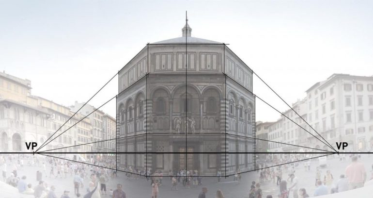
As shown by the quick proliferation of accurate perspective paintings in Florence, Brunelleschi likely understood (with help from his friend the mathematician Toscanelli), but did not publish, the mathematics behind perspective. Decades later, his friend Leon Battista Alberti wrote De pictura in 1435, a treatise on proper methods of showing distance in painting based on Euclidean (standard) geometry. However, these ideas remained the work of artists for around 100 years, when the architect Gerard Desargues rediscovered the notion of "points at infinity". Desargues advanced Brunelleschi's work by establishing the mathematics of not just lines and distance, but also that of conics, in paintings with vanishing points. Blaise Pascal, finding the writings of Desargues, was so inspired that he came up with the now famous Pascal's Theorem.
Unfortunately, just a few years later, Rene Descartes published a breakthrough work introducing cartesian coordinates, and work on projective geometry was mostly abandoned.
It was only in 1822, when mathematician Jean-Victor Poncelet published a foundational treatise on projective geometry, that interest in projective geometry reemerged.
Since then, it has revolutionized the foundations of algebraic geometry, influencing the works of Riemann, Dirac, Einstein, Bohr, etc.
Motivation
Draw a picture of a large, flat plain with a pair of railroad tracks running through it. It looks something like the picture below. When we draw a perspective picture like this, the parallel train tracks appear to actually meet at the horizon. Let’s change the rules of geometry a little so that this actually happens.

So, we define the projective plane initially as just the ordinary Real plane. But, like in our railroad, we want our parallel lines to eventually meet. So to our real plane, we add points, one for each set of parallel lines in the plane. We call these points the points at infinity. Thus, any two parallel lines intersect at the point at infinity corresponding to their slope.
We also add a line at infinity. It just passes through all of the points at infinity.
So, a normal line and the line at infinity intersect at the point at infinity corresponding to the slope of the normal line. So, every pair of distinct lines intersect at a single point.
And, every pair of distinct points has a single line passing through them. There's a notion of duality here: every two points determines a line, and every two lines determines a point. This is a key property of projective geometry.
If you can't visualize what this space looks like, don't worry! For now, as long as you can appreciate the duality of points and lines in projective space, you are on your way to understanding it.
Homothety
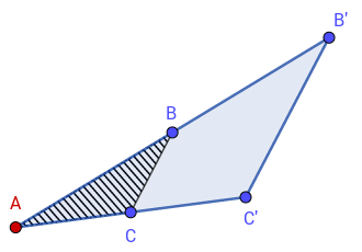
Before dealing with the projective plane, let's try to understand the duality between lines and points via projections in the standard plane. The simplest example of projection is the introduction of a vanishing point into the plane. A vanishing point is simply a point around which we project objects, like in the diagram below
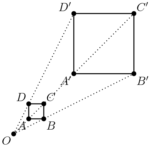
Point \(O\), the vanishing point, projects the square \(ABCD\) to the new square \(A'B'C'D'\). We call this projection homothety. The scale factor is the ratio \(\frac{OD'}{OD}\). We describe this homothety as \(H(O,D,D')\), or \(H\left(O,\frac{OD'}{OD}\right)\).
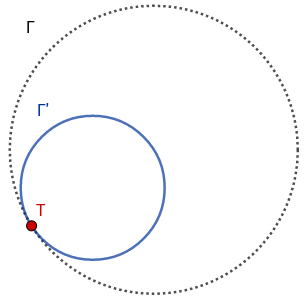
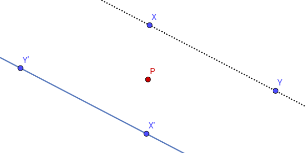
Given a vanishing point \((a,b)\) and a scale factor \(k\), \(H((a,b),k)\) sends point \((x,y)\) to \((k(x-a)+a,k(y-b)+b)\). Some examples of homothety are presented below.
- \(H(A,2)\) applied to \(\triangle ABC\):
- \(H(T,0.5)\) applied to a circle \(\Gamma\), with \(T\) on its circumference.
- \(H(P,-1)\) applied to the line \(XY\).
- The image of any object under homothety is similar to the object
- A homothety is uniquely defined by its action on two points
- The slope of a line under homothety is preserved.
- Angles are preserved under homothety
- For \(k\neq1\), the lines preserved by the homothety \(H(P,k)\) are the lines that go through \(P\)
- A shape with area \(A\) after homothety \(H(P,k)\) has area \(k^2A\), and a line segment with length \(l\) after the same homothety has length \(|k|l\).
As in art, the fun really begins when we introduce multiple vanishing points. How do multiple homotheties interact?
As a corollary of the above theorem, a translation composed with a homothety is a homothety.
The projective plane
Now that we've developed an appreciation for projection in the standard plane, let's extend the standard plane to build the projective plane. First, we'll develop a formal notion of a projective point (more commonly known as a homogenous coordinate).
Note that if we are given homogenous coordinates \([a;b;c]\), we can find the corresponding cartesian point by division as \(\left(\frac ac,\frac bc\right)\). But, the other way around isn't possible. Given a cartesian point \((x,y)\), there are multiple homogenous points corresponding to that cartesian point. For example, corresponding to \((1,1)\) are homogenous coordinates \([1;1;1]\), \([2;2;2]\), \([-5;-5;-5]\), etc.
That isn't great. Ideally, we'd want there to be exactly one homogenous coordinate for each cartesian coordinate. So how can we modify our space of homogenous coordinates to have this property?
The answer is simple: mods! We already used mods to a similar effect when constructing polynomial rings (see the Challenge Section on Week 11). Here, we observe the following phenomenon. If \((x,y)\) has homogenous representations \([a;b;c]\) and \([d;e;f]\), then \(\frac ac=\frac df\) and \(\frac bc=\frac ef\). If \(\lambda = \frac cf\), then $$[a;b;c]=[\lambda d;\lambda e;\lambda f]$$In other words, any two homogenous coordinates with the same cartesian coordinate representation are multiples of each other!
So, we set the following equivalence. \([a;b;c]\equiv[d;e;f]\) if there exists a number \(\lambda\) such that \(a=\lambda d\), \(b=\lambda e\), \(c=\lambda f\).
There is one issue with this construction: every homogenous coordinate has infinitely many equivalent homogenous coordinates, except for \([0;0;0]\). Thus, we disallow this as a homogenous coordinate. Why we do this will become obvious in a moment.
Now, we are ready to define the projective plane.
This is probably still very confusing. What is the difference between this and the normal cartesian coordinate system. How does this relate to the vanishing points that we talked about earlier? What does this space even look like? We'll answer all of these questions next.
Visualizing Projective Space
If we were to draw projective space, we might draw something like this:
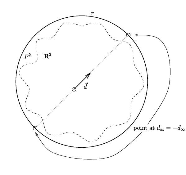
Inside the squiggly dotted line lies the real plane \(\mathbb R^2\). On the border of the real plane, we have the points at infinity, which we call \(d_\infty\). Each one corresponds to a possible direction of line, since any two parallel lines head in the same direction (however, each direction and the direction in the exact opposite direction have the same point at infinity: thus, \(d_\infty=d_{-\infty}\)). So the circle labeled \(r\) is really the "line at infinity" which goes through all of the points at infinity.
This visual should bother you. What does it mean for there to be a boundary on the plane. Doesn't the plane go off to infinity? There isn't any border! However, we are just building our intuition before we see the actual picture.
Let's go back to our construction of the projective plane via homogenous coordinates. What does the set of homogenous points that are equivalent to a points \([a;b;c]\) look like if we plotted them on a graph?
If you haven't seen linear algebra before, try drawing a 3D diagram, or perhaps using WolframAlpha to draw one for you. Once you do so, you'll see that the set is just the points on the line that goes through the origin \((0,0,0)\) and \((a,b,c)\)! In other words, the projective plane is the set of lines in 3D space that go through the origin.
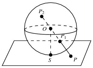
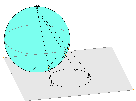
But how can we rectify this perspective with the ones we've discussed earlier? That's where projection (and hence the name projective plane) comes into play. In our 3D space, draw the plane \(w=1\) as in the diagram below. Then, each point \(P\) in the plane \(w=1\) corresponds to the line \(PO\) in projective space (where \(O\) is the origin). And, the points at infinity are represented by the lines parallel to the plane \(w=1\).
![]()
If this image still isn't clear, here's another way to see it. Add to the picture above the unit sphere in 3D space. Every line through the origin intersects this sphere at exactly two points. In fact, since the lines goes through the center of the sphere, projective space can be viewed as the space of diameters of the unit sphere.
Diameters are often identified by their endpoints. So what if we associate points in projective space with points on the sphere? Would that work? Almost. For any point \([x;y;z]\) on the unit sphere, the homogenous point \([-x;-y;-z]\) is also on the unit sphere and is equivalent to \([x;y;z]\). So we can define projective space in a new way.
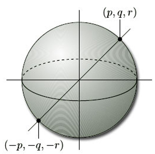
In other words, the projective plane can be viewed as half of the sphere, since we are removing half of the points.
Our new diagram is as follows: point \(P\) in the cartesian plane is represented by the line \(PO\), which is also represented by points \(P_1,P_2\) in the unit sphere.
We now have \(5\) ways of thinking about the projective plane.
- The cartesian plane with points at infinity and a line at infinity added in.
- The set of homogenous coordinates under an equivalence relation.
- The set of lines through the origin in 3D space.
- The projections of the origin onto a plane \(w=1\).
- The set of points on the unit sphere under an equivalence relation.
The more of these ways of thinking you master, the better your understanding of the projective plane will be.
- On the border of the cartesian plane
- The points at infinity are the points \([a;b;0]\), and the line at infinity is the set of points at infinity
- The points at infinity are the lines parallel to the \(x-y\) plane, and the line at infinity is just the \(x-y\) plane.
- The points at infinity are the projections that don't meet the plane \(w=1\), and the line at infinity is the set of these points.
- The points at infinity are the points on the unit sphere in the \(x-y\) plane, and the line at infinity is the unit circle in the \(x-y\) plane.
Solving the above exercise should test your understanding of the projective plane. Now, let's do some things with it!
Homogenous Polynomials
The projective plane is very useful because any two points determine a line, and any two lines determine a point. This symmetry leads to a cleaner way to handle line and conics than in Coordinate Geometry.
Suppose we take the standard formula for a line in the cartesian plane: \(ax+by+c=0\). If we replace \((x,y)\) with \([X;Y;Z]\), we get the formula $$a\frac XZ+b\frac YZ+c=0$$Multiplying by \(Z\), we get $$aX+bY+cZ=0$$This is called a homogenous polynomial, since all of the terms have the same degree (\(1\)).
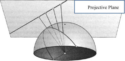
We can similarly homogenize a quadratic polynomial. \(ax^2+bxy+cy^2+dx+ey+f=0\) becomes $$aX^2+bXY+cY^2+dXZ+eYZ+fZ^2=0$$ As we can see, homogenizing a line gives us a plane in 3D space, as in the following diagram:
![]()
Now why would we want to homogenize polynomials? One of the great benefits is the following theorem:
Let's understand what this theorem means. It say, if we move any conic from the real plane to the projective plane, it becomes isomorphic to a circle. By isomorphic, we roughly mean, we can stretch or compress one shape to form the other (for example, a circle is isomorphic to an ellipse, since we can stretch the circle out. The circle is not isomorphic to a parabola, since the parabola has an open end.)
This is not an obvious theorem! In the real plane, ellipses, parabolas, and hyperbolas are all non-isomorphic (you can't transform any one of them into any other of them.) However, in the projective plane, they are all really just the same shape.
To see why this is the case, let's imagine the image of these conics on the sphere (our 5th way of imagining the projective plane.)
As the diagram above shows, a line through the origin in the cartesian plane is a great circle on the sphere. What about our conics?
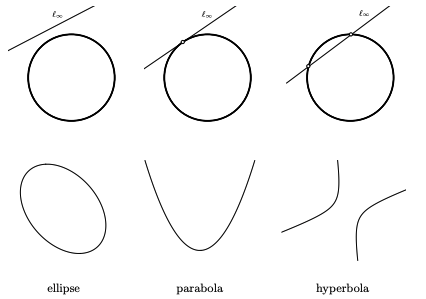
In the diagram above, \(l_\infty\) represents the line at infinity. If a circle on our sphere doesn't touch the line at infinity, as in the first example, the projection onto the real plane of the circle will be an ellipse, as in the following picture.
If we are in the second case, in which the circle touches the line at infinity at one point (as a tangent), the projection will be a parabola. And in the third case, where the line at infinity is a secant to the circle, the projection of the circle will be a hyperbola.
Another way of thinking about the differences between these \(3\) conics is as follows. In the projective space, the two "U"s in the hyperbola are glued together on each of their strands at the two points at infinity which they intersect at. The parabola's two strands intersect at one point at infinity. Thus, you can begin to imagine both of these shapes as very stretched out ellipses.
- \(x^2=1\)
- \(x^2-y^2=1\)
Duality
Now that we've developed the projective plane, we can formalize our understanding of the duality between lines and points.
With these definitions, we've associated every point in projective space with a line, and vice versa. This association has several nice properties that will formalize our understanding of duality.
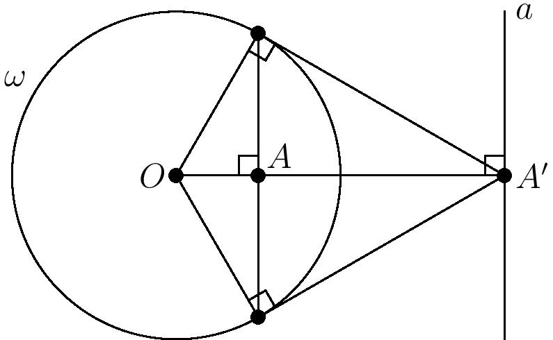
- If line \(l\) is the line at infinity, its pole is \(O\), whose polar is the line at infinity
- If \(O\) is on line \(l\), then the pole is the intersection of the line perpendicular to \(l\) through \(O\) with the line at infinity. And, the polar of this point is just \(l\)
- If neither of the above cases hold, then \(OA'\) has length \(0\lt d\lt\infty\), where \(A'\) is the closest point to \(O\) on line \(l\). Thus, \(A\) is the pole of \(l\) as defined above. And, the polar of \(A\) is the line that goes through \(A'\) that is perpendicular to \(OA'\). By standard geometry (prove it if it isn't obvious), the point closest to \(O\) on a line \(l\) satisfies \(OA'\perp l\).
- If \(l\) is the line at infinity, then \(p\) is a point at infinity, meaning that the polar of \(p\) is a line through the origin and the pole of \(l\) is the origin.
- If \(l\) goes through the origin, then the pole of \(l\) is the point at infinity perpendicular to \(l\). Thus, we just need to show that the polar of \(p\) is perpendicular to \(l\). If \(p\) is a point at infinity, the polar of \(p\) is the line perpendicular to \(l\) through the origin. If \(p\) is the origin, the polar is the line of infinity, containing the pole of \(l\). If \(p\) is any other point, the polar of \(p\) is a line perpendicular to \(l\).
- If \(l\) is any other line, then the situation is akin to the diagram above with \(l=a\) and \(p=A'\). Thus, the pole of \(a\) is \(A\) and the polar of \(A'\) is the line through \(A\) perpendicular to \(OA\).
Note that the incidence theorem implies that a point is on a line if and only if its polar contains the pole of the line (can you see why?). With the isomorphism and incidence theorems, we've established that the projective plane is dual, meaning that there is a one to one mapping between points and lines that preserves points being on lines. With self-duality, we gain a lot of power.
Self-duality implies that for any theorem in the projective plane that involves points, lines, concurrency (lines intersecting at the same point), and collinearity (points on the same line), the dual theorem, which is the theorem with lines and points switched, and concurrency and collinearity switched, is also true. Let's see a few examples of dual theorems.
\(X,Y\) being points at infinity imply \(AB\parallel DE\) and \(BC\parallel EF\). Consider the homothety \(H(P,B,E)\) (the homothety at \(P\) that sends \(B\) to \(E\)). Since homothety preserves slope, sends \(B\) to \(E\), and sends lines \(PA\) and \(PC\) to themselves, it must send \(A\) to \(D\) and \(C\) to \(F\). This implies that \(CA\parallel FD\) as homothety preserves slope, proving that \(Z\) is on the line of infinity.
We call the point of concurrency the center of perspective and the line of collinearity the axis of perspective.
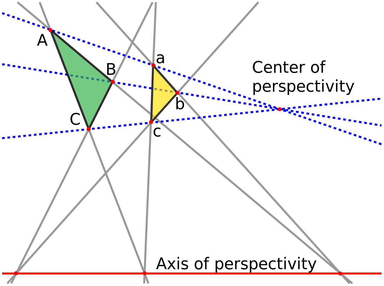
So what is the dual of Desargue's Theorem? It's just the converse!
The next example is a bit more relevant in contest mathematics.
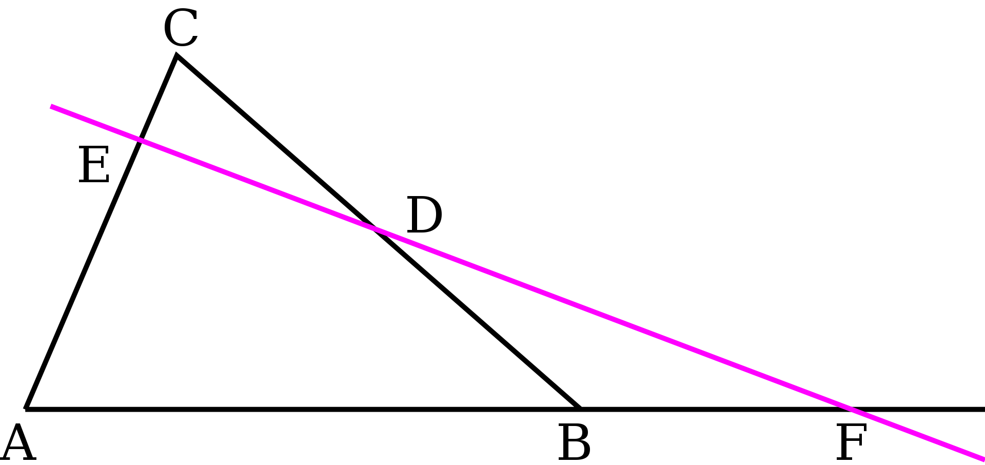
- If \(F\) is on line \(DE\), then the final homothety also keeps line \(DE\) fixed. Since points \(B,D,E\), which aren't collinear, are all fixed by the composition, the composition must be the identity. That means that the product of the scale factors must be \(1\). In other words, $$\frac{CD}{BC}\cdot\frac{AE}{EC}\cdot\frac{BF}{FA}=1$$
- If \(F\) is not on \(DE\), then \(F\) doesn't fix \(DE\), so the composition doesn't either. Since \(B\) is fixed by the homothety, the composition of the three homotheties must be a homothety centered at \(B\) with scale factor not equal to \(1\). Thus, $$\frac{CD}{BC}\cdot\frac{AE}{EC}\cdot\frac{BF}{FA}\neq1$$
The dual of Menelaus's Theorem is Ceva's Theorem, which says the following:
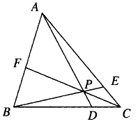
These theorems and homothety/projection as general tools are immensely valuable in geometry problems. Here's an example.
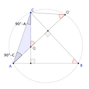
Note by right triangle properties that \(\angle Q'AC+\angle A=90^\circ\), and \(\angle QCA+\angle C=90^\circ\). Thus, $$\angle CQ'A=\angle Q'QC=\angle Q'AC+\angle QCA=180^\circ-\angle A-\angle C=\angle B$$Thus, by the Secant Angles Theorem, \(Q'\) lies on the circumcircle. So, if \(H_1,H_2,H_3\) are the reflections of point \(H\) over the sides \(BC\), \(CA\), \(AB\), they'd all lie on the circumcircle.
Next, let \(A',B',C'\) be the reflection of \(H\) over \(D,E,F\). Then, by right triangle properties$$\begin{aligned}\angle BCH+\angle ABC&=90^\circ\\\angle CBH+\angle ACB&=90^\circ\end{aligned}$$So, $$\angle BHC=180^\circ-\angle BCH-\angle CBH=\angle ABC+\angle ACB=180^\circ-\angle BAC$$Since \(HD=DA'\) and \(BD=DC\), \(BHCA'\) is a parallelogram, and thus \(\angle BHC=\angle BA'C\). So, \(\angle BA'C+\angle BAC=180^\circ\), and by the cyclic quadrilateral theorem, \(A'\) is on the circumcircle. Thus, \(A',B',C'\) are all on the circle.
Consider \(H(H,0.5)\). By definition, it maps \(A,B,C\) to \(P,Q,S\). By our work above, it maps \(H_1,H_2,H_3\) to \(K,L,M\) and \(A',B',C'\) to \(D,E,F\). Since all of these points are on the circumcircle, and the homothety of a circle is a circle, the theorem is proved.
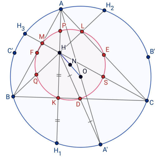
Moreover, since altitudes of \(DEF\) are perpendicular bisectors of \(ABC\), \(H'\) is the point of intersection of the perpendicular bisectors of \(ABC\), which implies that \(H'=O\). This proof also implies the following relations:$$HG=2GO,\;ON=NH,\;OG=2GN,\;NH=3GN$$
The Euler line also happens to contain a lot of other special points in the triangle. Look at this link for more details.