Week 3 Notes
More about Combinations
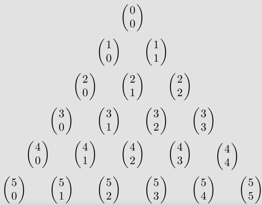
Our first topic for this week will be exploring combinations and their applications. From here on out, we'll adopt a new notation for combinations: we'll write \(n\choose k\) to represent \(_nC_k\).
Perspective 1: Pascal's Triangle
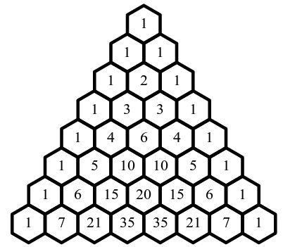
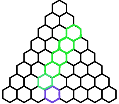
Suppose I have the following triangle:
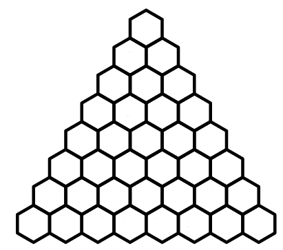
I start at the top hexagon, and at each step, I can hop to the hexagon to my bottom right, or to my bottom left, as in the diagram below
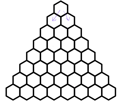
Then, I repeat this process, hopping down the triangle at each step. Now suppose I pick some hexagon in my triangle
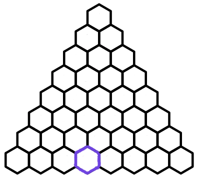
And I ask, how many ways are there for me to hop from the top hexagon to my chosen hexagon? Below is one possible way for me to hop from the top hexagon to the chosen hexagon:
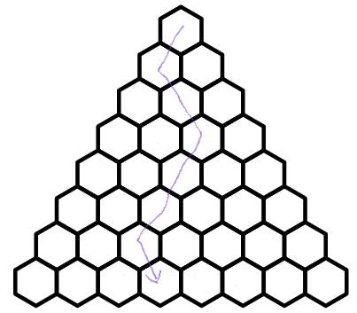
To compute the number of ways, I make a few key observations:
- Every path from the top hexagon to the purple hexagon will take exactly \(7\) hops.
- Every path from the top hexagon to the purple hexagon will take \(4\) hops to the bottom left.
So how many paths satisfy these properties? Well, the idea is simple: we have \(7\) hops, and \(4\) of them must be to the left. So, we simply need to choose \(4\) of the \(7\) hops to be to the left, set the rest to be to the right, and we are golden. So, the answer is \({7\choose 4}=35\).
We can generalize this logic to find the number of paths to any hexagon in our triangle. Here's a diagram showing how that's done:
This triangle is known as Pascal's triangle and has many special properties. For starters, let's look back at the purple hexagon. Is there another way we can compute the number of paths to it?
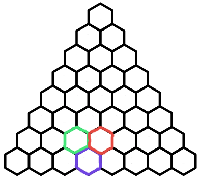
Observe that every path to the purple hexagon must go through exactly one of the green hexagon and the red hexagon. In other words, the number of paths to the purple hexagon is the sum of the number of paths to the red and green hexagons. This gives us the following formula for any \(k\lt n\):$${n\choose k}+{n\choose k+1}={n+1\choose k+1}$$This is called Pascal's identity. If we apply Pascal's identity to the red hexagon, we get the following diagram:
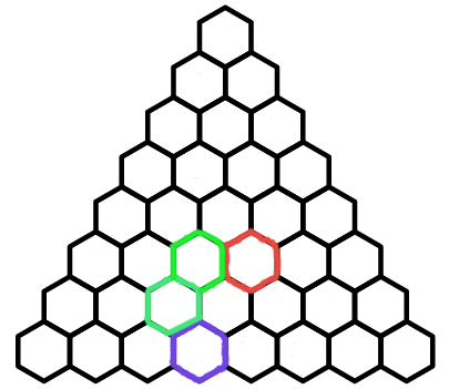
If we keep replacing the red hexagons with Pascal's Identity, we eventually get this diagram:
This tells us that the sum of the paths to each of the green hexagons is the number of paths to the purple hexagon. In equation form, this is $$\sum\limits_{i=k}^n{i\choose k}={n+1\choose k+1}$$This formula is known as the Hockey Stick Identity.
Perspective 2: Binomial Distribution
Suppose I have a biased coin (a coin that flips heads with probability \(p\) instead of \(0.5\), and tails with probability \(1-p\)), and I flip it \(3\) times. What is the probability of getting exactly \(2\) heads?
There are three different ways this can happen: \(HHT\), \(HTH\), and \(THH\). Each of these ways are mutually exclusive, so we can consider them individually.
- \(HHT\): Since each flip is independent, the probability of getting this outcome is \(p\cdot p\cdot (1-p)\)
- \(HTH\): the probability of this outcome is \(p\cdot(1-p)\cdot p\).
- \(THH\): the probability of this outcome is \((1-p)\cdot p\cdot p\)
The answer is no. In each of the three cases, there is one tails and two heads. So the probability of each occuring is the same. So the final formula is \(3\cdot p^2\cdot(1-p)\).
So why were there \(3\) possibilities? Each possibility was given by placing the \(2\) heads in the sequence of \(3\) flips. There are \({3\choose 2}=3\) ways to do this.
We can now generalize our problem. Suppose I flip my biased coin \(n\) times. What is the probability of getting exactly \(x\) heads? Well, for any one of the valid outcomes, the probability is \(p^x\cdot(1-p)^{n-x}\). And, there are \(n\choose x\) valid outcomes. So, the probability is $${n\choose x}p^k(1-p)^{n-x}$$This is known as the binomial distribution, and is useful in many probability problems. The following diagram summarizes our work so far:
So how is this related to Pascal's triangle?
Perspective 3: Polynomials
Consider the polynomial \((x+y)^n\). There are coefficients \(c_n,\ldots,c_0\) such that $$(x+y)^n=c_nx^n+c_{n-1}x^{n-1}y^1+\ldots+c_1x^1y^{n-1}+c_0y^n$$How do we find \(c_n,\ldots,c_0\)? Well, let's try some examples
| \((x+y)^0\) | \(1\) |
| \((x+y)^1\) | \(1x+1y\) |
| \((x+y)^2\) | \(1x^2+2xy+1y^2\) |
| \((x+y)^3\) | \(1x^3+3x^2y+3xy^2+1y^3\) |
| \((x+y)^4\) | \(1x^4+4x^3y+6x^2y^2+4xy^3+1y^4\) |
| \((x+y)^5\) | \(1x^5+5x^4y+10x^3y^2+10x^2y^3+5xy^4+1y^5\) |
| \((x+y)^6\) | \(1x^6+6x^5y+15x^4y^2+20x^3y^3+15x^2y^4+6xy^5+1y^6\) |
| \((x+y)^7\) | \(1x^7+7x^6y+21x^5y^2+35x^4y^3+35x^3y^4+21x^2y^5+7xy^6+1y^7\) |
Does this look vaguely familiar? If not, click this. The coefficients are just the elements of Pascal's tree!
And this should make sense: the coefficient of \(x^ay^b\) should be \(a+b\choose a\) since we are choosing which \(a\) of the \(a+b\) \((x+y)\) terms we are choosing \(x\) from, and choosing \(y\) from the rest.
Thus, we have the following theorem: $$(x+y)^n=\sum\limits_{k=0}^n{n\choose k}x^ky^{n-k}$$This is known as the binomial theorem. If we let \(x=p\) and \(y=1-p\), we get $$1^n=\sum\limits_{k=0}^n{n\choose k}p^k(1-p)^{n-k}$$The right hand side of this formula is the binomial probability of getting \(k\) heads from \(n\) tosses. That's pretty cool!
Now, let \(x=y=1\). Then, we have $$2^n=\sum\limits_{k=0}^n{n\choose k}$$We can generate a lot of cool formulas by playing around with \(x,y\), but this should be enough for now.
Note: I don't want you to memorize these formulas. Rather, understand the three perspectives. Mathematicians view these three perspectives as three different ways of seeing the same thing, and you'll become very strong at probability problems if you're able to do the same thing!
Introduction to Statistics
Statistics is the study of data, and for this week, we'll look at some basic ways of understanding data.
I'm doing a research project where I ask every student in my class their height. Here is the data I got (in inches)
| \(60\) | \(60\) | \(62\) | \(63\) | \(64\) | \(64\) | \(64\) | \(66\) | \(66\) | \(67\) | \(68\) | \(69\) | \(72\) | \(73\) | \(80\) |
What can I tell from this information?
Measures of Centrality
The first thing I might want to know is, what is the middle of the data? There are a few different ways of measuring the "middle" of data.
Mean
The most obvious way of finding the middle is taking the average of the data, otherwise called the mean of the data. If I have \(n\) values of data, which I call \(x_1,\ldots, x_n\), the mean is defined as follows:$$\overline x=\frac1n\sum\limits_{k=1}^nx_k$$For our example, the mean is approximately \(66.53\).
The mean is a nice statistic because it is easy to calculate, and tells us what the middle of the data looks like, but it has an issue. If I have some outliers in my data (numbers that are much larger/smaller than the rest of the numbers), they affect the mean a lot. In our example, the \(6'8"\) individual dragged the mean from \(65.57\) to \(66.53\), almost an entire inch!
If we want a way of finding the middle that is less affected by outliers, we can use the next measure of centrality.
Median
Suppose I surveyed employees at company Boogle about their salaries, and received the following data (in thousands of dollars):
| \(24\) | \(25\) | \(28\) | \(28\) | \(31\) | \(33\) | \(240\) |
The mean of this data set is \($58,429\). This is silly, of course. This salary is much higher than all but one employee's income. Is this really the best measure of centrality?
In this case, we want a measure of centrality which is affected less by outliers (like the \($240,000\) salary). The median works as follows:
- If there is an odd number of data points, pick the value right in the middle of the data set.
- If there is an even number of data points, take the average of the two middle data points
Mode
The median, too, has its flaws. Suppose I had some data on the weights of students in a class (in lbs):
| \(105\) | \(108\) | \(110\) | \(112\) | \(136\) | \(136\) | \(140\) | \(143\) |
In this case, the median is \(124\) pounds. But, no student is near that weight. And that's probably because our data contains the weight of both boys and girls. A data set like this is called bimodal, since it looks like two datasets glued together. In this case, the median doesn't do a great job finding the center of the data. Can we do better?
The mode of the data is the most common data point. In this example, since \(136\) appears twice, it is the most common data point, and thus is the mode. The mode works best when we have a lot of data, since there will be some repetition, and the mode will measure that well.
In summary, we have seen three measures of centrality. Often, we compute all \(3\) of them, and compare their results to understand our data. For example, if the mean is much greater than the median, we say that the data is right-skewed, meaning that there is likely some outliers on the right side of the data. If the mean is much less than the median, we say that the data is left-skewed, meaning that there is likely some outliers on the left side.
Measures of Variability
We saw how to measure the middle of a data set. But how do we measure how spread out it is?
| \(1\) | \(5\) | \(9\) | \(9\) | \(9\) | \(13\) | \(17\) |
| \(7\) | \(8\) | \(9\) | \(9\) | \(9\) | \(10\) | \(11\) |
Range
The range is very simple: it is the difference of the biggest value minus the smallest value. In the example above, the range of the first dataset is \(17-1=16\), and the range of the second data set is \(11-7=4\).
The range has the same issues that the mean does: it is far too sensitive to outliers. For example, the range of this dataset is \($216,000\), which isn't a good measure of that data set. Can we do better?
Interquartile Range
The Interquartile range is a modification to the range which is a bit more resilient to outliers. Like the median, we have slightly different rules for calulating it if the data set has even or odd number of values
- If the data set has an even number of values, let \(Q_1\) be the median of the lower half of the data, and \(Q_3\) be the median of the upper half. The IQR is \(Q_3-Q_1\).
- If the data set has an odd number of values, remove the median from the data set, and then calculate the interquartile range.
The IQR also let's us compute outliers ourselves! We call the value \(Q_1-1.5\cdot\text{IQR}\) the lower whisker of the data set, and \(Q_3+1.5\cdot\text{IQR}\) the upper whisker. Any data not between the two whiskers is considered an outlier, and is thus removed from the data set.
To represent the information presented by the median, IQR, and the whiskers, we can draw a box plot.
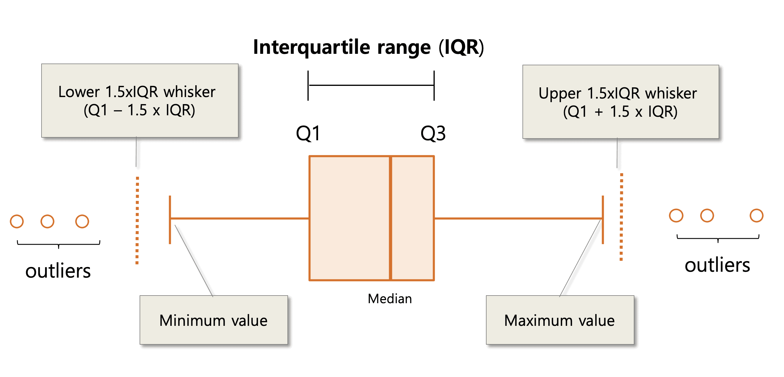
The minimum of the data is the smallest non-outlier data point, and the maximum of the data is the largest non-outlier data point.
Variance
Finding outliers with IQR sounds like a great idea! However, there is an issue. Why have we chosen \(1.5\)? The answer is rather unfortunate: it seems to work okay. When the IQR outlier rule was developed in the 1970s, it seemed to work well on the datasets of the time, but modern datasets have shown that the IQR rule can fail in a lot of cases. For this reason, most statisticians rely on variance for studying variability.
The idea is that we are measuring how far from the mean each data point is, and averaging their squares. The standard deviation \(\sigma\) is defined as the square root of variance.
The main issue with variance is that it is hard to compute by hand. However, here's a little shortcut to make it a bit easier to compute.$$\sigma^2=\frac1n\left(\sum\limits_{k=1}^nx_k^2-\left(\sum\limits_{k=1}^nx_k\right)^2\right)$$
| \(1.90\) | \(3.00\) | \(2.53\) | \(3.71\) | \(2.12\) | \(1.76\) | \(2.71\) | \(1.39\) | \(4.00\) | \(3.33\) |
Challenge: Graph Theory
Graphs are combinatorial objects that are hugely important in today's world. As such, we will cover just the basics in this section.
A (undirected) graph is just a collections of objects, which we call nodes, and edges, which are connections between pairs of nodes. For example, we can use a graph to show the six New England states, and which ones border each other.
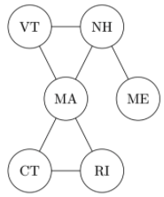
The degree of a node is the number of nodes connected to it. For example, the degree of Vermont is \(2\) as it is connected to New Hampshire and Massachussetts.
- If each node has degree \(4\), how many edges are there in the graph?
- Is it possible for half of the nodes to have degree \(5\) and the other half have degree \(4\)?
- If every two nodes are connected, how many edges are there
- Since each node has degree \(4\), and there are \(10\) nodes, the total number of edges is \(4\cdot10=40\), right? Well, we've double counted, since each edge is connected to \(2\) nodes. So, the number of edges is \(\frac{40}2=20\).
- Since \(5\) nodes have degree \(5\), they contribute \(25\) edges, and the other \(5\) nodes with degree \(4\) contribute \(20\) edges. Thus, there are \(45\) edges, but we've double counted. So, there are \(22.5\) edges. This isn't possible, so there can't be such a graph.
- Since there are \(n\choose2\) possible pairs of nodes in a graph with \(n\) nodes, the number of edges in this graph is \({10\choose2}=45\)
With this exercise, you should be able to see that the sum of degrees of the nodes in a graph is twice the number of edges, and that the maximal number of edges in a graph with \(n\) nodes is \(n\choose2\). In particular, this implies that the number of nodes with odd degree must be even.
Paths
Many of the real world examples motivating graphs involve travel. Nodes can be viewed as destinations, and edges as routes to travel.
But what if we wanted to travel between nodes with no direct route (in graph terms, edge) between them? We can travel along multiple paths!
To get from Maine to Rhode Island, you can travel from Maine, to New Hampshire, to Massachussetts, to Rhode Island. We call a series of edges that be travelled consecutively in this way a path.
In fact, the path from Maine to Rhode Island we mentioned isn't the only path (can you find another?), but it is the minimal path. A minimal path is a path from a start node to an end node that takes a minimal number of edges.
A cycle is a path that starts and ends at the same node. A graph is called connected if there exists a path connecting any two nodes in the graph.
A simple path is a path that doesn't cross any node twice
A connected graph with no simple cycles is called a tree. Trees have a lot of special properties, as we'll discover.
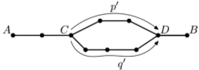
Thus, the path that first travels from \(C\to D\) along \(p'\), and then from \(D\) to \(C\) along \(q'\) is a cycle. Moreover, since \(p'\) and \(q'\) don't touch any of the same nodes besides \(C\) and \(D\) (otherwise \(D\) wouldn't be the first meeting point), this cycle is simple, a contradiction.
Now suppose that our graph satisfies the property that every two nodes \(A,B\) has exactly one simple path between them. Then, the graph is obviously connected. Now suppose there is a simple cycle \(e_1,\ldots,e_n\). Then, the path \(e_n,e_{n-1},\ldots,e_2\) is a simple path from \(C\) to \(D\), where \(e_1\) is an edge from \(C\) to \(D\). This means that there are two simple paths from \(C\) to \(D\), a contradiction.
The following exercise requires induction, so if you haven't seen it before, wait till Week 12 before attempting this exercise.
- Any connected graph with \(n\) nodes has at least \(n-1\) edges
- Any graph with \(n\) nodes and at least \(n\) edges has a simple cycle
- Any tree with at least \(2\) nodes has at least \(2\) nodes of degree \(1\)
There is so much more to learn about graphs. Feel free to explore further (and share what you've learned!)